Quickstart
Using the API Wrapper
With ngspicepy installed, you can import it using
import ngspicepy as ng
The library gives you access to several functions. First, you need to load a netlist. You can do so by specifying the filename that contains the netlist:
ng.load_netlist('circuit.net')
The extension doesn’t matter. Any text file containing a valid SPICE netlist will work. The function also accepts other ways to import netlist. Consult the documentation for more information.
Next you may want to run a simulation, say a DC simulation where the voltage of source V1 is varied from 0V to 10V in steps of 0.1V.
ng.run_dc('v1 0 10 0.1')
Currently, there are functions for AC, DC, TRAN and OP analyses. The functions provided check the input arguments for correctness since ngspice, at times, crashes when given wrong commands. For other types of analyses, you can directly run a valid ngspice command using,
ng.send_command('dc v1 0 10 0.1')
For the list of available commands, please consult the ngspice manual.
Next you can get the results. A simulation generates several vectors. You can get a list of these vector names using,
vecs = ng.get_vector_names()
where vecs contains a list of strings. Suppose you’re interested in
the voltage at node ‘1’. The name of the corresponding vector is ‘v(1)’. You
can get it’s contents using,
vec_data = get_data('v(1)')
If you want to get all of the data,
vecs_data = get_all_data()
Using the Netlist class
With ngspicepy installed you can import Netlist from is as:
from ngspicepy import Netlist
To plot the results import matplotlib and numpy as well using the command
import matplotlib.pyplot as plt
import numpy as np
The Netlist class gives you the acces to several functions to carry out simulation and get the data. Suppose you want to perform a TRAN analysis with the netlist for the circuit in the file name ‘CS-Amp.cir’ Then the first step to carry out is load the netlist as:
amp = Netlist('CS-Amp.Cir')
The extension doesn’t matter. Any tex file containg a valied SPICE netlist will work. Next, you want the initial time step to be ‘1u’ and and the simulation to stop at ‘10m’. You can set the parameter using the set_simu function as:
amp.setup_sim('tran', tstep='1u', tstop='10m')
After setting up the parameters you just need to run the simulation as:
amp.run()
For now the process of simulation setup and run has been completed. Now you can run the simulation number of times and extract the vectors associated with the plot names. In order to get the various vectors associated with TRAN analysis simply type:
amp.get_vectors_names('tran1')
You can also access each of these vectors individually by specifying the plot names. If no plot name is specified it gets the vector of the latest plot. The vectors associated with TRAN analysis are ‘time’, ‘nin’, ‘nout’. Each of these can be accessed as:
amp.get_vector('time')
amp.get_vector('nin')
amp.get_vector('nout')
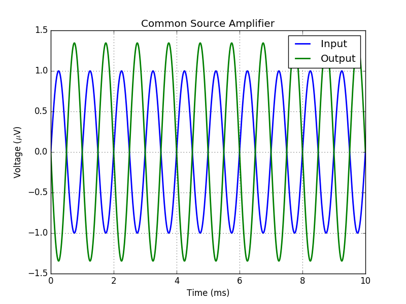
Now, you can plot the results using matplotlib
plt.plot(t * 1e3, 1e6 * v_in_small_signal, linewidth=2)
plt.plot(t * 1e3, 1e6 * v_out_small_signal, linewidth=2)
plt.legend(['Input', 'Output'])
plt.xlabel('Time (ms)')
plt.ylabel('Voltage ($\mu$V)')
plt.title('Common Source Amplifier')
plt.grid()
plt.show()
